The ZLOOKUP function is a unique feature introduced by Modern Functions Update (MFU) that does not exist in any version of Excel. You can now run it for free on your Excel from 2007 onward, including 365 and 2024 versions.
Description
The ZLOOKUP function searches for a value in the first column of a range and returns a value from another column in the same row. It is designed as a simpler, more intuitive alternative to VLOOKUP, with a syntax that makes it easier to use.
Unlike VLOOKUP, ZLOOKUP:
- Does not require the lookup column to be the first column
- Uses separate lookup and return ranges
- Has exact match as the default behavior
- Does not break when columns are inserted or deleted
Think of it as a lightweight, straightforward lookup function that works the way you’d expect it to.
This is particularly useful for:
- Simple lookups: Find a value in a list and return a corresponding value
- Data analysis: Match IDs to names, products to prices, etc.
- Reporting: Pull related data from different columns
- Data validation: Verify if a value exists in a list
Syntax
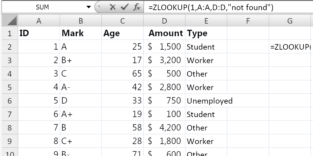
=ZLOOKUP(lookup_value, lookup_array, return_array, [if_not_found])
| Argument | Description |
|---|---|
lookup_value | Required. The value to search for. |
lookup_array | Required. The range or array to search. Must be a single row or column. |
return_array | Required. The range or array from which to return the corresponding value. Must be the same size as lookup_array. |
[if_not_found] | Optional. The value to return if no match is found. If omitted, returns #N/A. |
Important Notes
ZLOOKUPuses exact match by default – no need to specify0orFALSE.- The
lookup_arrayandreturn_arraymust be the same size. - The
lookup_arraycan be any column or row – it does not need to be the first column. - If no match is found,
ZLOOKUPreturns the value specified in[if_not_found]or#N/A. - The function is case-insensitive: “APPLE” and “apple” are treated as the same value.
- The function works with text, numbers, dates, and other data types.
Examples
Basic Usage
If you have product IDs in column A and prices in column B:
=ZLOOKUP("P001", A2:A100, B2:B100)
Returns the price from column B where the ID in column A matches “P001”.
With Custom “Not Found” Message
=ZLOOKUP("P001", A2:A100, B2:B100, "Product not found")
Returns the price if found, or "Product not found" if the ID doesn’t exist.
Lookup to the Left
Unlike VLOOKUP, ZLOOKUP can look up to the left because the lookup and return ranges are separate:
=ZLOOKUP("Smith", B2:B100, A2:A100)
Finds “Smith” in column B and returns the corresponding value from column A.
With Cell References
If the value to look up is in cell E2:
=ZLOOKUP(E2, A2:A100, B2:B100, "Not found")
With Dates
=ZLOOKUP(TODAY(), A2:A100, B2:B100, "No data for today")
Nested ZLOOKUP
To perform a two-way lookup (similar to INDEX-MATCH-MATCH):
=ZLOOKUP(D2, B6:B17, ZLOOKUP(C3, C5:G5, C6:G17))
This looks for “Gross Profit” in column B and “Qtr1” in the top row, then returns the value at the intersection.
ZLOOKUP: The Perfect Balance Between Simplicity and Power
If you’ve ever struggled with Excel’s lookup functions, ZLOOKUP is the function you’ve been waiting for. It sits in the sweet spot between the outdated VLOOKUP and the powerful but sometimes overwhelming XLOOKUP.
Why ZLOOKUP is Better than VLOOKUP
Let’s face it – VLOOKUP has limitations that have frustrated Excel users for decades:
- ❌ The lookup column must be the first column – if your data isn’t structured that way, you’re stuck
- ❌ Column index numbers break when you insert or delete columns
- ❌ Approximate match is the default – a mistake that leads to wrong results
- ❌ Cannot look to the left
ZLOOKUP solves all of this:
- ✅ Lookup column can be anywhere
- ✅ Uses separate lookup and return ranges – no column index numbers
- ✅ Exact match is the default – no more accidental wrong results
- ✅ Looks left, right, anywhere
Practical Use Cases
| Scenario | Formula |
|---|---|
| Product lookup | =ZLOOKUP(F2, A2:A100, B2:B100, "Not found") |
| Employee search (left lookup) | =ZLOOKUP(F2, C2:C100, B2:B100) |
| Price lookup | =ZLOOKUP(E2, A2:A100, C2:C100) |
| Date lookup | =ZLOOKUP(TODAY(), A2:A100, B2:B100) |
| Two-way lookup | =ZLOOKUP(D2, B6:B17, ZLOOKUP(C3, C5:G5, C6:G17)) |
| Handle missing values | =ZLOOKUP(E2, A2:A100, B2:B100, "No data") |
Notes
- ✅ Fully tested – The implementation in Modern Functions Update works reliably.
- ✅ The function is fully compatible with Excel 2007, 2010, and all later versions.
- ℹ️
ZLOOKUPis a unique MFU feature not found in any Excel version. - ℹ️ The function uses exact match by default – no need for a match mode argument.
- ℹ️ The
lookup_arraycan be any column or row – it does not need to be sorted. - ℹ️ The function is case-insensitive: “Apple” and “apple” are treated as the same value.
- ⚠️ If there are duplicate values in
lookup_array,ZLOOKUPreturns the first match found.
See Also
IFNA – Handles #N/A errors gracefully
XLOOKUP – More advanced lookup function with additional features
XMATCH – Returns the position of a value