The XLOOKUP function was officially introduced with Excel 2021, but thanks to Modern Functions Update (MFU) you can now run it on your Excel 2007, 2010, 2013, 2016 and 2019 versions. It works exactly as its original Microsoft counterpart.
Description
The XLOOKUP function searches a range or an array for a specified value and returns the corresponding value from another range in the same row. It is designed as the modern replacement for VLOOKUP, HLOOKUP, and many INDEX-MATCH combinations.
Think of it as the lookup function that can finally do everything you always wished VLOOKUP could do:
- Search in any direction – Left, right, up, or down. The lookup column doesn’t need to be on the left.
- Never break when inserting columns – Because you specify separate lookup and return ranges.
- Built-in error handling – No more wrapping formulas in
IFERROR. - Return multiple values – A single formula can return an entire row of results.
- Search from first or last match – Find the first occurrence or work your way from the bottom up.
If you’ve ever been frustrated by VLOOKUP’s limitations, XLOOKUP is the solution you’ve been waiting for.
Syntax
=XLOOKUP(lookup_value, lookup_array, return_array, [if_not_found], [match_mode], [search_mode])
| Argument | Description |
|---|---|
lookup_value | Required. The value to search for. |
lookup_array | Required. The array or range to search. |
return_array | Required. The array or range to return values from. |
[if_not_found] | Optional. Value to return if no match is found. If omitted, returns #N/A. |
[match_mode] | Optional. Specify the match type (see table below). Default is 0 (exact match). |
[search_mode] | Optional. Specify the search direction (see table below). Default is 1 (first to last). |
Match Modes
| Value | Behavior |
|---|---|
| 0 | Exact match. If none found, return #N/A. This is the default. |
| -1 | Exact match. If none found, return the next smaller item. |
| 1 | Exact match. If none found, return the next larger item. |
| 2 | Wildcard match where *, ?, and ~ have special meaning. |
Search Modes
| Value | Behavior |
|---|---|
| 1 | Search from first item to last. This is the default. |
| -1 | Reverse search from last item to first. |
| 2 | Binary search (requires lookup_array sorted ascending). |
| -2 | Binary search (requires lookup_array sorted descending). |
Examples
Basic Lookup
Find the price of a product based on its ID:
=XLOOKUP(E2, A2:A100, B2:B100)
Returns the price from column B where the ID in column A matches the value in E2.
Custom “Not Found” Message
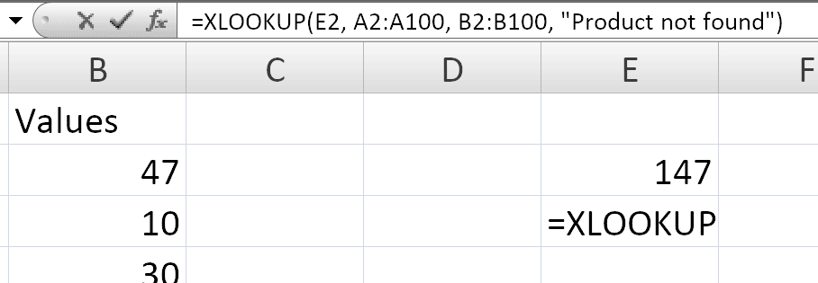
If the value isn’t found, return a friendly message instead of #N/A:
=XLOOKUP(E2, A2:A100, B2:B100, "Product not found")
Lookup to the Left (VLOOKUP can’t do this)
Find an employee name based on their ID, where the ID column is to the right of the name column:
=XLOOKUP(F2, C2:C100, B2:B100, "Employee not found")
With VLOOKUP, you would need to restructure your data. XLOOKUP handles this effortlessly.
Return Multiple Columns
Instead of writing three separate formulas, write one that returns an entire row of data:
=XLOOKUP(L4, A2:A201, B2:J201, "Not found")
This spills results across multiple cells horizontally – one formula, nine results.
Reverse Lookup (Find the Last Match)
Need the most recent transaction for a customer rather than the first? Set search_mode to -1:
=XLOOKUP(G2, A2:A201, B2:J201, "No transactions", 0, -1)
This searches from the bottom up, returning the last matching row.
Find the Date of a Minimum or Maximum
If you have dates in column A and expenditures in column B, find the date of the minimum or maximum expenditure:
=XLOOKUP(MIN(B:B), B:B, A:A)
=XLOOKUP(MAX(B:B), B:B, A:A)
Nested XLOOKUP (Two-Way Lookup)
Perform both a vertical and horizontal match – similar to INDEX-MATCH-MATCH:
=XLOOKUP(D2, B6:B17, XLOOKUP(C3, C5:G5, C6:G17))
This looks for “Gross Profit” in column B and “Qtr1” in the top row, then returns the value at the intersection.
Sum Values Between Two Lookup Values
Use two XLOOKUP functions to return a range, then sum it:
=SUM(XLOOKUP(B3, B6:B10, E6:E10) : XLOOKUP(C3, B6:B10, E6:E10))
XLOOKUP returns a range reference, so this works like SUM(E7:E9).
XLOOKUP vs VLOOKUP – Key Differences
Practical Use Cases
| Scenario | Formula |
|---|---|
| Product lookup | =XLOOKUP(F2, A2:A100, B2:B100, "Not found") |
| Employee search (left lookup) | =XLOOKUP(F2, C2:C100, B2:B100) |
| Customer last transaction | =XLOOKUP(G2, A2:A201, B2:J201, , 0, -1) |
| Multiple columns at once | =XLOOKUP(L4, A2:A201, B2:J201) |
| Date of min/max value | =XLOOKUP(MAX(B:B), B:B, A:A) |
| Two-way lookup | =XLOOKUP(D2, B6:B17, XLOOKUP(C3, C5:G5, C6:G17)) |
| Partial match (wildcard) | =XLOOKUP("Smith*", A2:A100, B2:B100, , 2) |
Notes
- ✅ Fully tested – The implementation in Modern Functions Update works identically to Microsoft’s original function introduced in Excel 2021.
- ✅ The function is fully compatible with Excel 2007, 2010, and all later versions.
- ℹ️ If the
lookup_valueis omitted, XLOOKUP returns blank cells it finds inlookup_array. - ℹ️ All ranges must be the same size.
- ⚠️ If using binary search modes (2 or -2), the
lookup_arraymust be sorted correctly, otherwise invalid results will be returned.