The FILTER function was officially introduced with Excel 2021, but thanks to Modern Functions Update (MFU) you can now run it on your Excel 2013, 2016 and 2019 versions. It works exactly as its original Microsoft counterpart.
While older versions of Excel, 2007 and 2010, should use FILTERX instead.
The FILTER function filters a range of data based on one or more conditions you define. It returns a dynamic array of matching values that automatically updates when the source data changes.
Think of it as the perfect replacement for manual filtering using dropdowns. Instead of clicking through menus, you write a formula that automatically shows you exactly what you need.
This is particularly useful for:
- Creating live reports: Show only the data that meets specific criteria
- Dashboard building: Display filtered data that updates automatically
- Data analysis: Extract subsets of data for further analysis
- Report generation: Create dynamic lists that respond to user inputs
- Working with large datasets: Focus on relevant information without manual filtering
Syntax
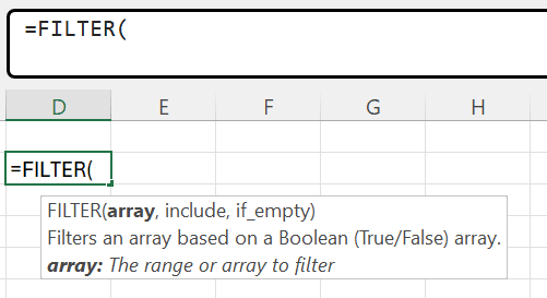
=FILTER(array, include, [if_empty])
| Argument | Description |
|---|---|
array | Required. The range or array to filter. |
include | Required. A Boolean array (TRUE/FALSE) of the same height or width as the array. |
[if_empty] | Optional. The value to return when no data meets the criteria. If omitted, returns an empty array. |
Important Notes
- The
includeargument must be a Boolean array (TRUE/FALSE) – generally created using logical expressions - The
arrayandincludearguments must be the same size FILTERis a dynamic array function – results spill into adjacent cells automaticallyFILTERdoes not work inside an Excel Table- For older Excel versions (2007 & 2010), use
FILTERXinstead ofFILTER
Examples
Basic Filtering – Single Condition
To filter the table A4:B19 and return only rows where the Category is “Fruit”:
=FILTER(A4:B19, C4:C19="Fruit")
Returns the entire rows from A4:B19 where the category in column C is “Fruit”.
Filtering Multiple Columns
To filter data from columns B and C only (excluding the category column):
=FILTER(B4:C19, C4:C19="Fruit")
Returns only columns B and C from the rows where the category is “Fruit”.
Multiple Conditions (AND)
To filter rows where Category is “Fruit” and Sales > 30:
=FILTER(A4:B19, (C4:C19="Fruit") * (B4:B19>30))
The multiplication (*) works like the AND operator; both conditions must be TRUE.
Multiple Conditions (OR)
To filter rows where Category is “Fruit” OR Sales > 30:
=FILTER(A4:B19, (C4:C19="Fruit") + (B4:B19>30))
The addition (+) works like the OR operator; at least one condition must be TRUE.
Using Cell References for Criteria
To filter based on a value in another cell (E2):
=FILTER(A4:B19, C4:C19=E2)
Change the value in E2 to update the filter result instantly.
Custom “No Results” Message
To show a custom message when no data matches:
=FILTER(A4:B19, C4:C19="Fruit", "No records found")
This returns "No records found" instead of an error.
Sorting Filtered Results
To filter and sort the results:
=SORT(FILTER(A4:B19, C4:C19="Fruit", "No records found"), 2, -1)
This filters for “Fruit” and sorts the results by column 2 in descending order.
Extracting Unique Values with Criteria
To extract unique values that meet criteria:
=UNIQUE(FILTER(A4:A19, C4:C19="Fruit"))
Returns unique values from column A where the category in column C is “Fruit”.
Using FILTERX in Older Versions
For Excel 2007 and 2010, use FILTERX with the exact same syntax:
=FILTERX(A4:B19, C4:C19="Fruit", "No records found")
FILTERX is specifically designed for compatibility with older Excel versions and works identically to FILTER in newer versions.
Practical Use Cases
| Scenario | Formula |
|---|---|
| Filter by category | =FILTER(Data, Category="Fruit") |
| Filter by multiple criteria (AND) | =FILTER(Data, (Category="Fruit") * (Sales>30)) |
| Filter by multiple criteria (OR) | =FILTER(Data, (Category="Fruit") + (Sales>30)) |
| Filter with cell reference | =FILTER(Data, Category=E2) |
| Filter with custom message | =FILTER(Data, Category="Fruit", "No records") |
| Filter and sort | =SORT(FILTER(Data, Category="Fruit"), 2, -1) |
| Unique filtered values | =UNIQUE(FILTER(A:A, B:B="Fruit")) |
| Count filtered results | =COUNTA(FILTER(A:A, B:B="Fruit")) |
Common Problems
| Problem | What It Means | What To Do |
|---|---|---|
| #NAME? error | Excel doesn’t recognize FILTER/FILTERX | Install Modern Functions Update |
| #SPILL! error | The spill range is blocked by existing data | Clear the cells where the result wants to spill |
| #VALUE! error | Inconsistent or mismatched range sizes | Ensure array and include arguments are the same size |
| #CALC! error | No data meets criteria and if_empty omitted | Add an if_empty argument or check your criteria |
| #REF! error | Formula references a closed workbook | Open the workbook containing the referenced array |
Notes
- ✅ Fully tested – The implementation in Modern Functions Update works identically to Microsoft’s original function introduced in Excel 2021
- ✅ The function is fully compatible with Excel 2007, 2010, and all later versions
- ⚠️ For older versions (2007 & 2010), use
FILTERXinstead ofFILTERfor compatibility - ℹ️ The
FILTERfunction is a dynamic array function – results spill into adjacent cells - ℹ️ The
FILTERfunction is case-insensitive – “Fruit”, “FRUIT”, and “fruit” are treated the same - ℹ️ For AND logic, use
*between conditions; for OR logic, use+