The FILTERX function was introduced by Modern Functions Update (MFU) in order to allow users of older Excel versioni, namely 2007 and 2010, to use a function similar to FILTER. Thanks to FILTERX you can now use a very similar FILTER-like function close to its original Microsoft counterpart.
FILTER was officially introduced with Excel 2021, but thanks to Modern Functions Update (MFU) you can now run it on your Excel 2013, 2016 and 2019 versions. If you are on Excel 2007 or 2010, please use FILTERX instead.
Description
The FILTERX function filters a range of data based on one or more conditions you define, returning matching rows from the source data. It is the compatible alternative to FILTER for Excel 2007 and 2010.
Think of it as a powerful filtering tool that works exactly like FILTER, but with a syntax that older Excel versions can understand.
This is particularly useful for:
- Creating live reports – Show only the data that meets specific criteria
- Dashboard building – Display filtered data that updates automatically
- Data analysis – Extract subsets of data for further analysis
- Working with large datasets – Focus on relevant information without manual filtering
Syntax
=FILTERX(array, criteria_range, criteria, [if_empty])
| Argument | Description |
|---|---|
array | Required. The range or array to filter. |
criteria_range1 | Required. The range to evaluate against the first condition. |
criteria1 | Required. The condition to apply to criteria_range1. |
| Optional. The value to return when no data meets the criteria. |
Important Notes
- The
arrayand allcriteria_rangearguments must be the same number of rows. FILTERXsupports multiple conditions – simply add more range/criteria pairs.- The
[if_empty]argument is always the last argument. - If no
[if_empty]is provided and no data matches, the function returns a blank cell.
Examples
Basic Filtering – Single Condition
Using the sample data, to filter all rows where the Type is “Student”:
text
=FILTERX(A:E, E:E, "Student")
Returns all rows from columns A to E where the value in column E equals “Student”.
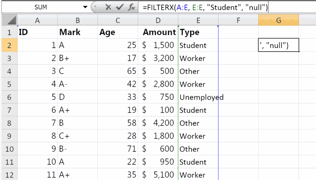
With “No Results” Message
To show a custom message when no data matches:
=FILTERX(A:E, E:E, "Student", "null")
Returns filtered data or "null" if no students are found.
Using Cell References for Criteria
To filter based on a value in another cell (G1):
=FILTERX(A:E, E:E, G1)
Change the value in G1 to update the filter result instantly.
Filtering with Numeric Criteria
To filter rows where Age is greater than 30:
=FILTERX(A:E, C:C, ">30")
Returns all rows where the Age in column C is greater than 30.
Practical Use Cases
| Scenario | Formula |
|---|---|
| Filter by type | =FILTERX(A:E, E:E, "Student") |
| Filter by type with no results message | =FILTERX(A:E, E:E, "Student", "null") |
| Filter by cell reference | =FILTERX(A:E, E:E, G1) |
| Numeric criteria | =FILTERX(A:E, C:C, ">30") |
Notes
- ✅ Fully tested – The implementation in Modern Functions Update works reliably in Excel 2007 and 2010.
- ✅ The function is fully compatible with Excel 2007, 2010, and all later versions.
- ℹ️
FILTERXuses a range/criteria pair syntax, unlikeFILTERwhich uses a Boolean array. - ℹ️ The
[if_empty]argument is always the last argument. - ⚠️ All criteria ranges must have the same number of rows as the
array.